Cell Ranger6.4, printed on 04/13/2025
By default, a .cloupe gene expression dataset includes all barcodes called as cells by
Cell Ranger's cell caller.
The default clusters and projections in a .cloupe file are derived from this set of cells.
However, it may be more useful to only analyze a subset of these cells. For example, it may be desirable to more precisely screen out possible cell multiplets, dead cells, or cells with low diversity. Alternatively, it may be preferable to focus on a particular type of cell, or even remove a particular cell type from an analysis.
For these reasons, Loupe Browser 5.0 and later provides an interactive filtering and reclustering workflow. In a few short steps, it is possible to identify cells of interest, and then compute a Louvain clustering and t-SNE projection over these cells. Loupe Browser 5.1 and later additionally supports the generation of a UMAP projection.
| Loupe Browser 6.2 supports reclustering for GEX (Gene Expression) data in GEX + Antibody Capture, GEX + CRISPR Guide Capture, and GEX + ATAC datasets. |
To enter the reclustering workflow, select Categories mode, and choose any category. A Recluster button will appear above the cluster names and clicking it will launch a separate window for the workflow:
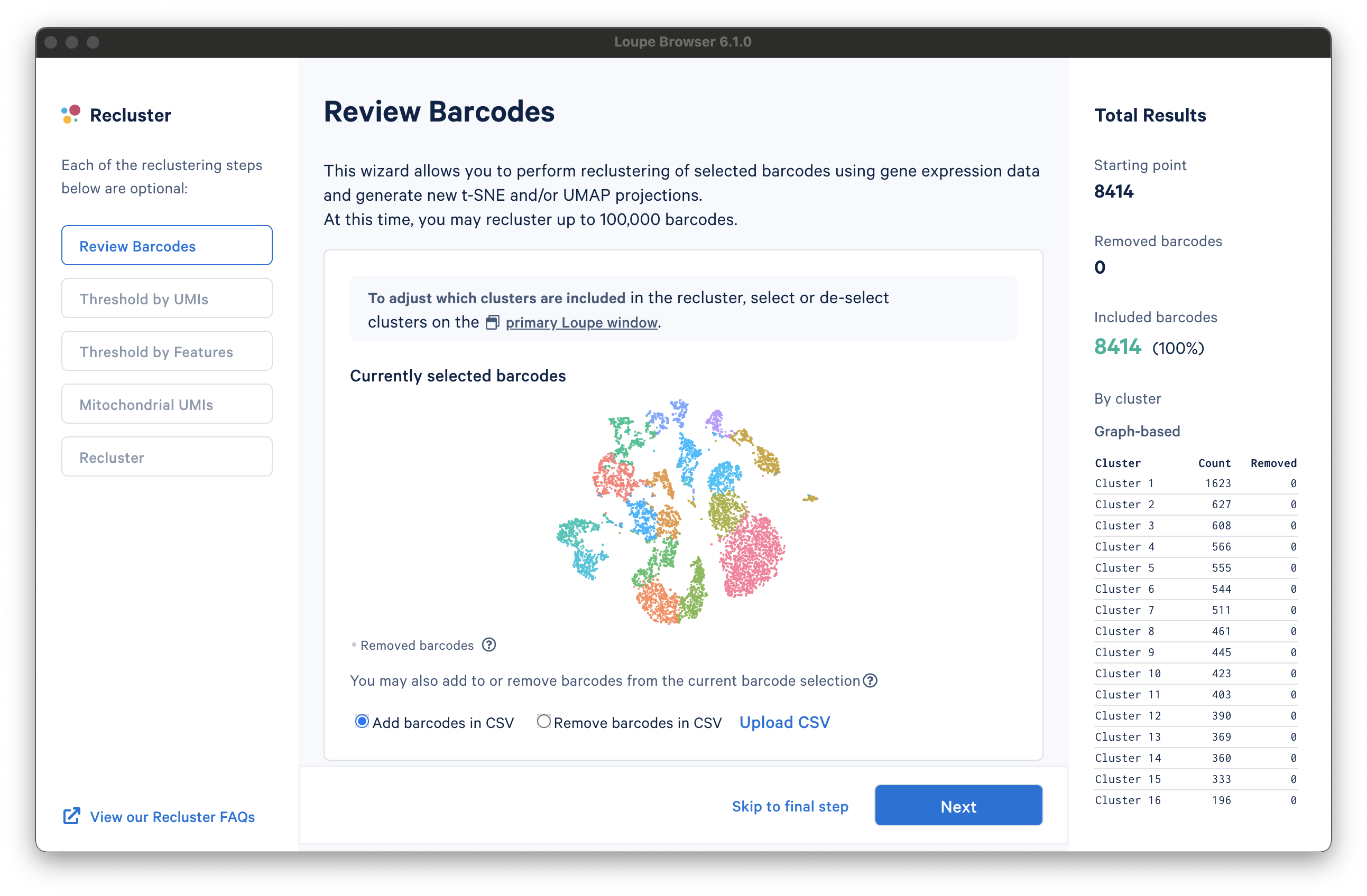
There are three columns for all steps in the workflow. The leftmost column shows the current progress through the workflow steps. It is possible to advance or go back to any step in the workflow at any time. The middle column contains the tooling for the active step. The rightmost column shows statistics about which barcodes have been removed. On the bottom of the Recluster window, there are buttons to advance to the next step or skip to the final step. Each step in the workflow is described in the sections below.
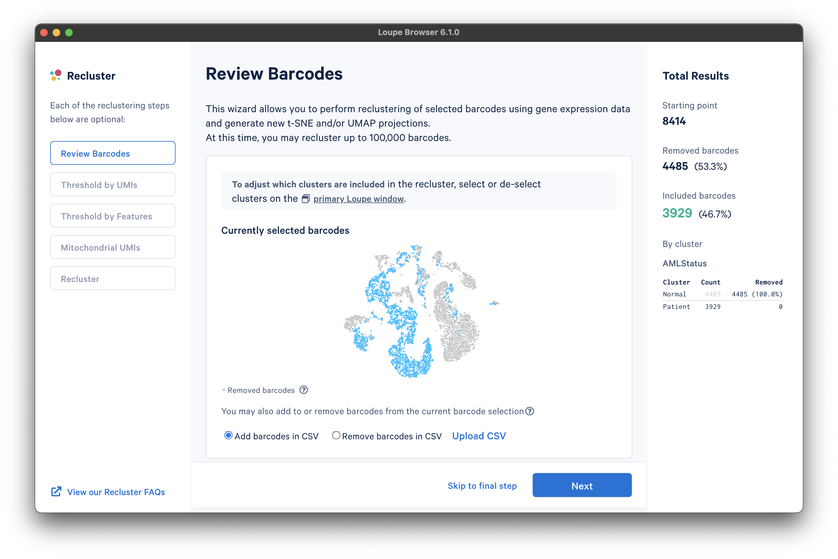
The first step, Review Barcodes, allows an initial filtering by either whole clusters, or a barcode list. It is connected to the main window; changing the category in the main window will change the active category in the reclustering workflow. By selecting or de-selecting clusters in the main window, it is possible to either include or exclude entire clusters of barcodes from downstream analysis. The image below illustrates the built-in AML Tutorial dataset. With the "AMLStatus" category selected and the "Normal" cluster de-selected, as shown below:
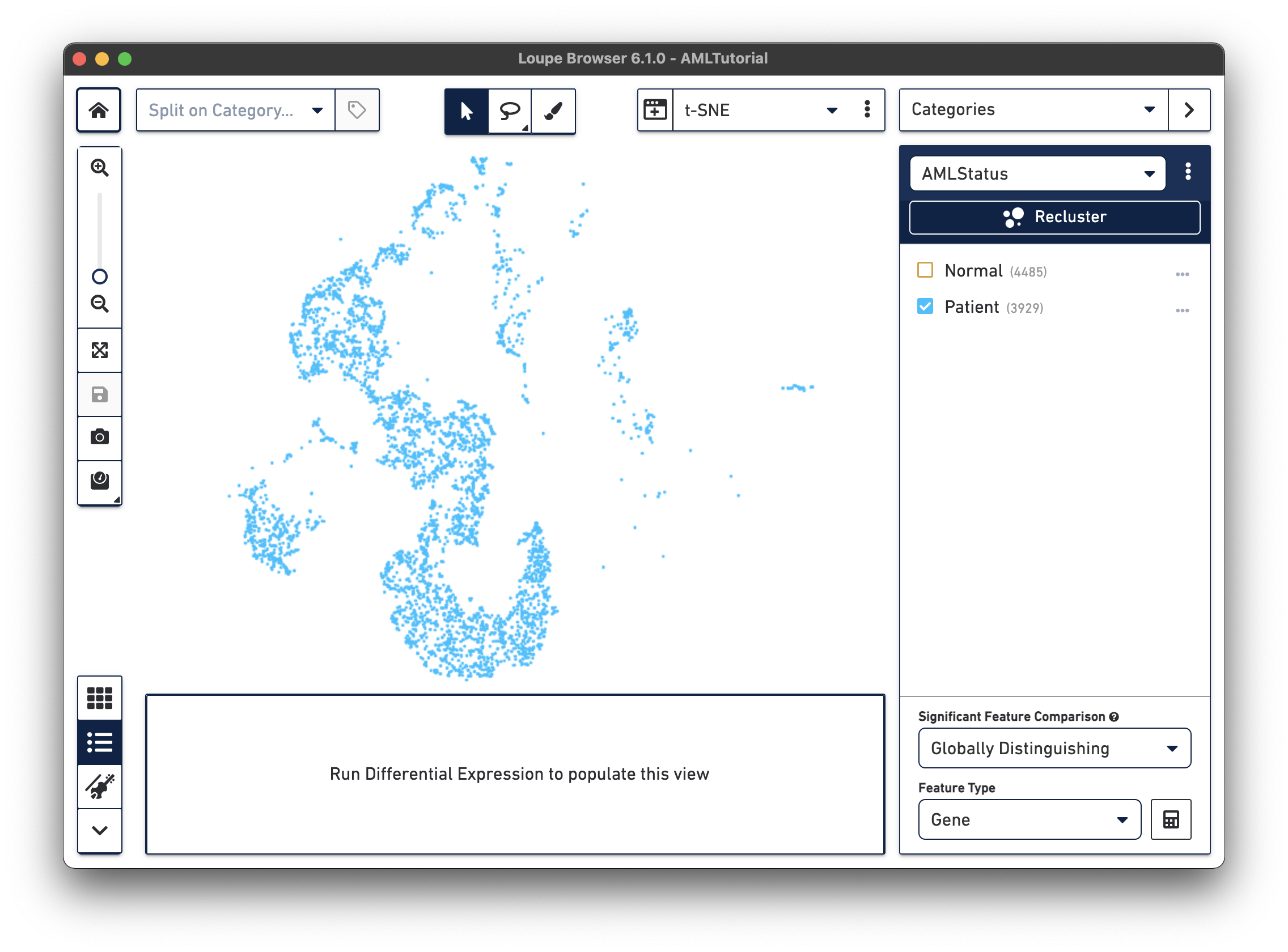
The reclustering workflow will respond in kind, removing the "Normal" barcodes:
It is also possible to filter by custom categories, such as those created with the lasso tools, quantitative filters, boolean filters, or CSV import. It is recommended that these categories be created prior to initiating the reclustering workflow.
Finally, for finer-grained control, or to filter by lists defined by external algorithms, it is possible to either explicitly add or remove a set of barcodes by clicking the Upload CSV link below the plot.
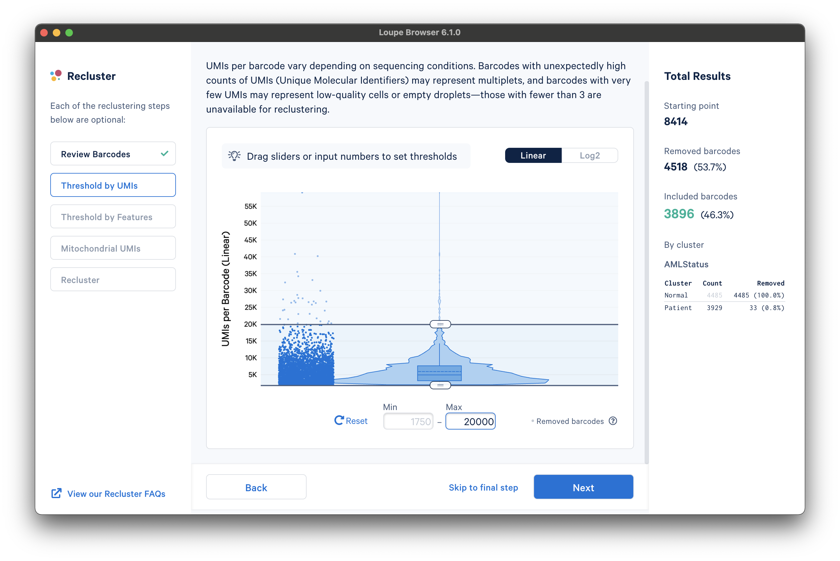
The next step is to threshold by UMI count. This step shows a violin plot of UMI counts of the currently selected barcodes. Moving the sliders at the top and bottom of the distribution will remove barcodes from outside the range. It is also possible to enter numerical values explicitly, or see the distribution on a log plot. For the purpose of this tutorial, an upper UMI count limit of 20,000 UMIs per barcode on the linear scale will be used, as shown below:
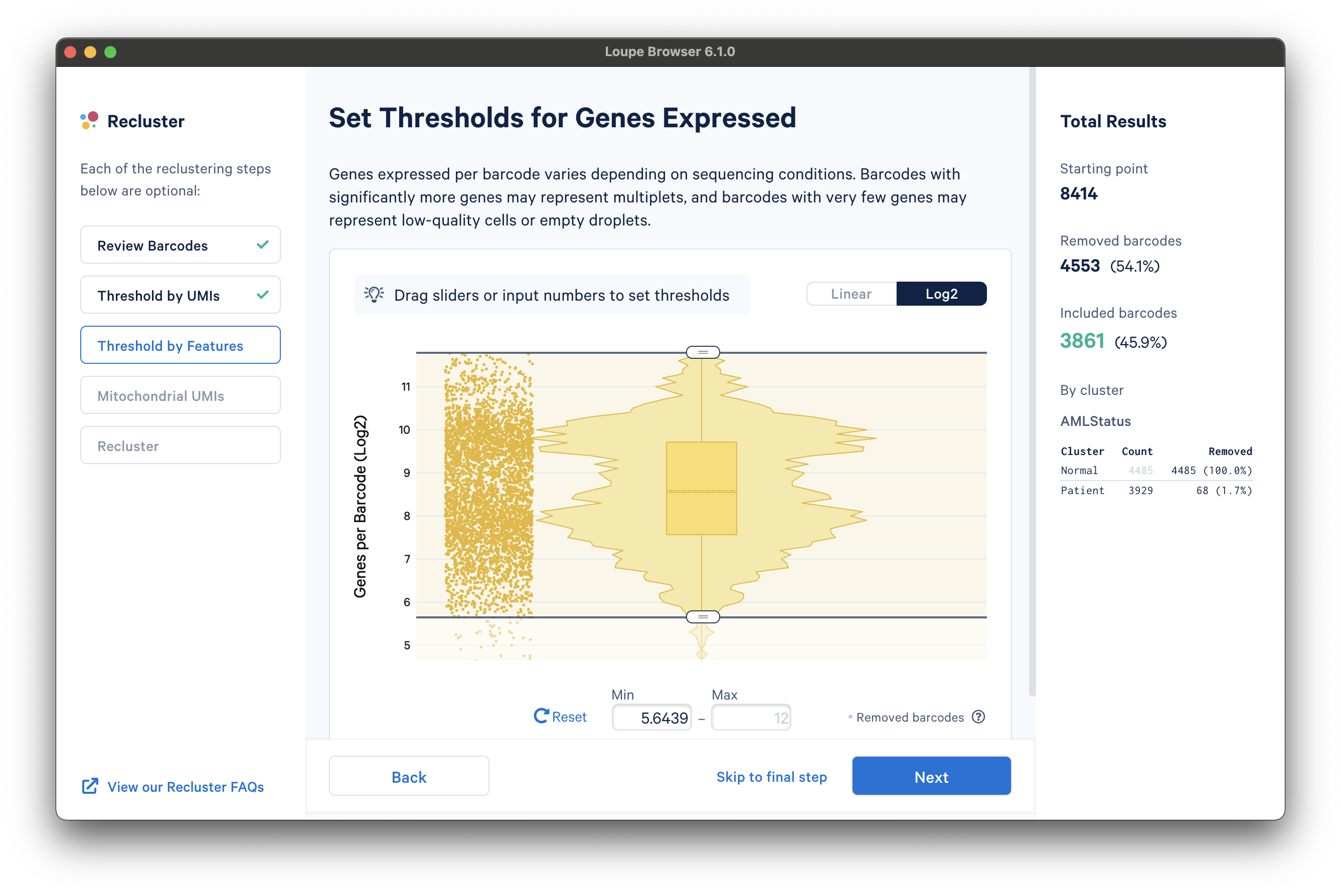
The next step is to threshold by a distinct number of detected features. For gene expression datasets (even with Feature Barcoding), this will be the number of distinct genes found for each barcode. Depending on the experiment, barcodes with anomalously low or high numbers of distinct features may be undesirable. For the purpose of this tutorial, a lower feature count bound of 50 features per barcode on the linear scale (5.6439 equivalent on log scale) will be used, as shown below:
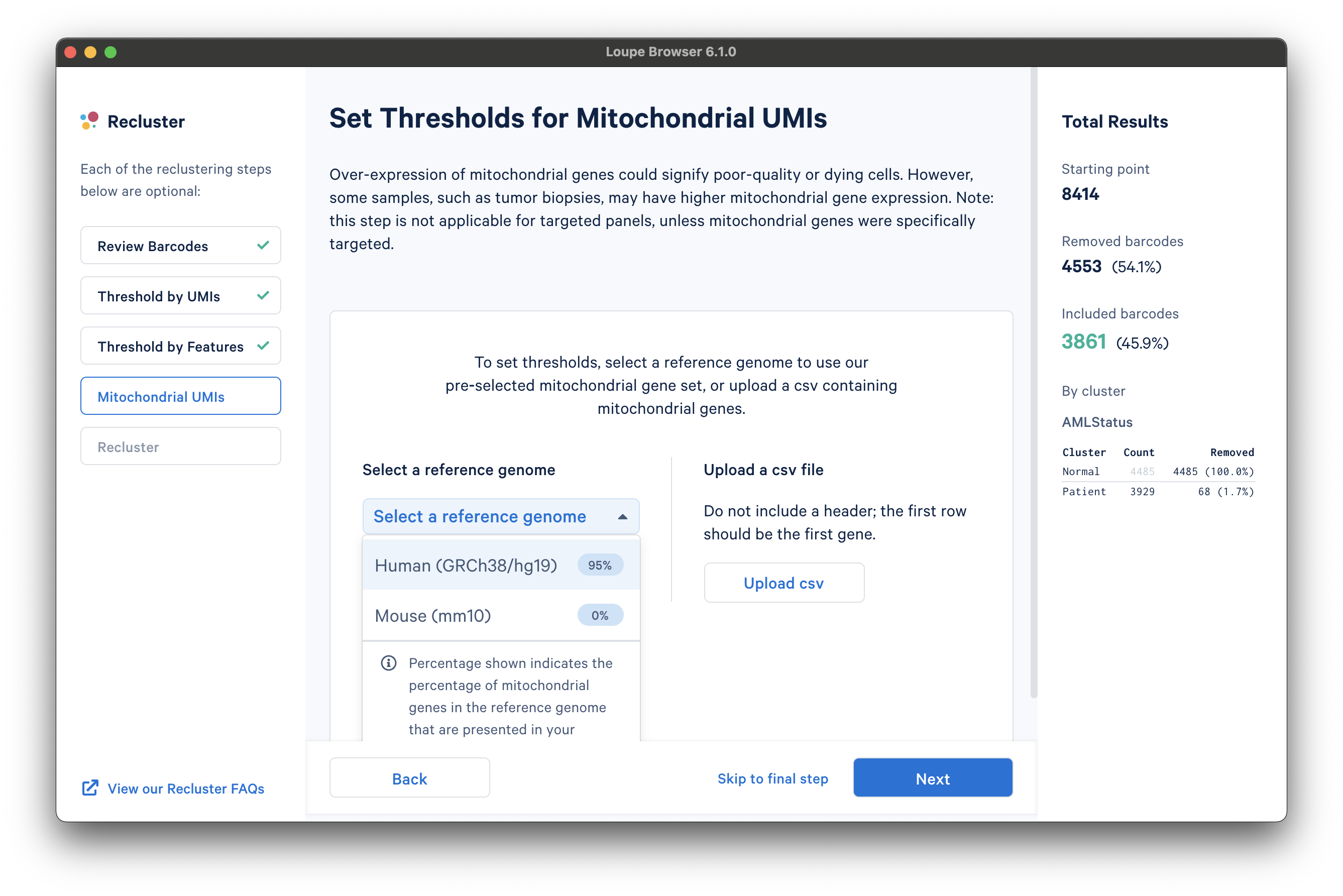
The next step is to filter cells by mitochondrial fraction -- the percentage of UMIs per barcode associated with mitochondrial genes. This step requires either the selection of a predefined reference (human or mouse), or uploading the set of mitochondrial genes for a custom reference. This step is not applicable for targeted panels, unless mitochondrial genes were specifically targeted.
To select from the list of pre-recognized references, click the Select a reference genome drop-down menu. The options will show the percentage of mitochondrial genes in the reference that are present in the dataset. The AML Tutorial dataset is a human dataset, with most mitochondrial genes present. Note that the human reference list of mitochondrial genes are prefaced with "MT-" (e.g., "MT-ATP6", "MT-CO1", etc.), which may not match all gene names used in custom references.
To specify your own list of mitochondrial genes, create a text-based file with a ".csv" file extension that has no header and lists one gene per row. We can parse the custom reference GTF file to find the exact names used for the mitochondrial genes.
For example, using the GTF file from the example custom Rhesus macaque reference on a Linux computer, we will look at the contents of the GTF file (the -S flag makes it easier to see the columns):
zcat Macaca_mulatta.Mmul_10.105.gtf.gz | less -S
The file output should look similar to (use the arrow keys to scroll right, up, and down):
#!genome-build Mmul_10
#!genome-version Mmul_10
#!genome-date 2019-02
#!genome-build-accession GCA_003339765.3
#!genebuild-last-updated 2019-12
1       ensembl gene    8231    26653   .       -       .       gene_id "ENSMMUG00000023296"; gene_version "4"; gene_source "ensembl"; gene_biotype "protein_coding";
1       ensembl transcript      8231    26653   .       -       .       gene_id "ENSMMUG00000023296"; gene_version "4"; transcript_id "ENSMMUT00000032773"; transcript_version "4"; gene_source "ensembl"; gene_biotype "protein_coding"; transcript_source "ensembl"; transcript_biotype "protein_coding";
1       ensembl exon    26570   26653   .       -       .       gene_id "ENSMMUG00000023296"; gene_version "4"; transcript_id "ENSMMUT00000032773"; transcript_version "4"; exon_number "1"; gene_source "ensembl"; gene_biotype "protein_coding"; transcript_source "ensembl"; transcript_biotype "protein_coding"; exon_id "ENSMMUE00000287659"; exon_version "3";
...
MT      RefSeq  gene    3259    4213    .       +       .       gene_id "ENSMMUG00000065372"; gene_version "1"; gene_name "ND1"; gene_source "RefSeq"; gene_biotype "protein_coding";
...
Next, we will look for the mitochondrial genes in the GTF file. You can look at the .fai index of the genome FASTA file to list out the contig names. For this macaque example, the mitochondrial contigs are called "MT". This command searches for records where the contig "MT" is in the 1st column and record type "gene" is in the 3rd column, and saves results in a text file. Note that the exact usage of single (') and double (") quotation marks in these commands is important for successfully parsing the file!
zcat Macaca_mulatta.Mmul_10.105.gtf.gz | awk '($1 == "MT") && ($3 == "gene")' > macaque-mito-genes.txt
Finally, we parse the text file to only keep a list of mitochondrial gene names and save the results in a CSV file. The first awk command prints only the column with gene names. The remaining cut, sort, and uniq commands clean up the formatting (e.g., remove quotation marks and duplicate row names).
cat macaque-mito-genes.txt | awk 'FS="; " {print $3}' | cut -d" " -f2 | cut -d'"' -f2 | sort | uniq > macaque-mito-intermediate.txt
This particular example still contains rows with "RefSeq" and "gene" - these can be removed in a text editor like nano or with awk commands:
cat macaque-mito-intermediate.txt | awk '!/RefSeq/' | awk '!/gene/' > macaque-mito-genenames.csv
The output looks like this:
ATP6
ATP8
COX1
COX2
COX3
CYTB
ND1
ND2
ND3
ND4
ND4L
ND5
ND6
Now, the CSV file can be used in Recluster by clicking the Upload csv button.
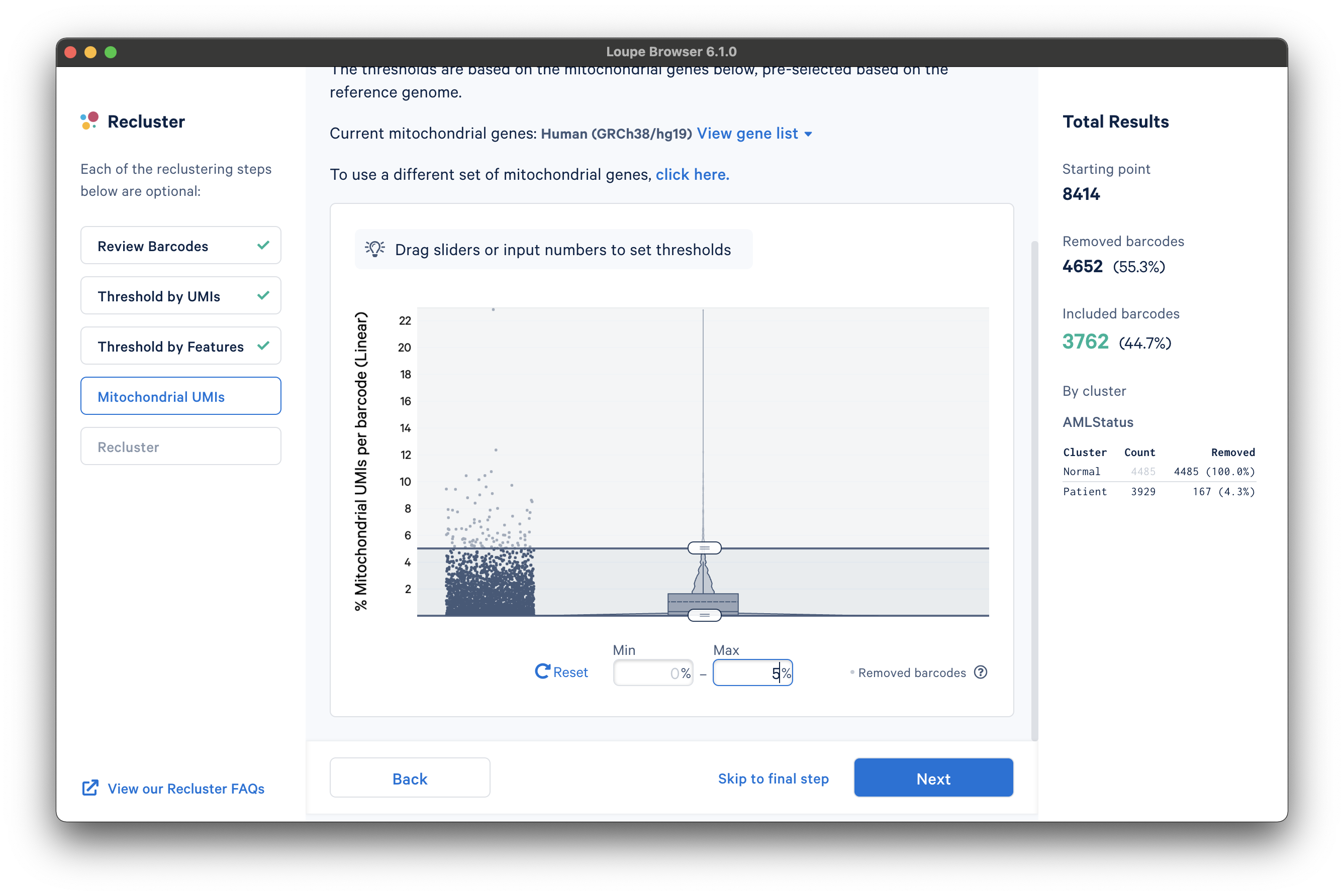
After selecting a reference or uploading a gene list, another violin plot and slider will be visible. In this tutorial, we set a mitochondrial fraction upper bound of 5%. This threshold will vary depending on your experiment.
With the filtering steps done, the next step is to determine the type of plot to generate. It is possible to generate a t-SNE or UMAP projection. Note that selecting both will double the processing time.
Under the Adjust reanalyze parameters (for advanced users) drop-down menu, it is possible to enter custom parameters for the dimensionality reduction used for clustering, or the parameters for generating the t-SNE and UMAP plots respectively. For each parameter, there are detailed instructions if you select Learn more. Defaults are recommended, and no action is necessary if the default values are acceptable. In this tutorial, a UMAP projection with default reanalyze parameters was selected.
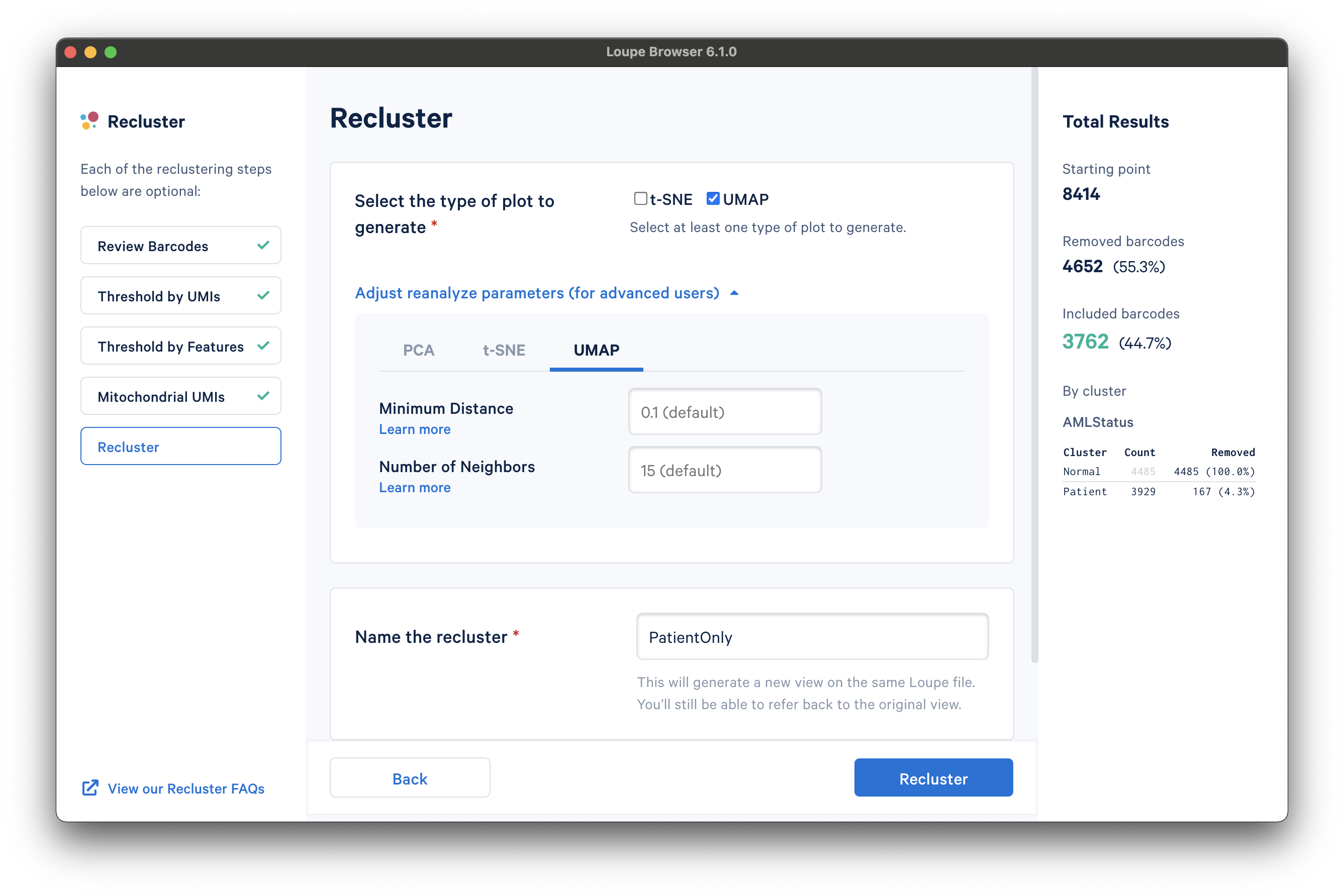
Finally, the last step is to name the recluster dataset. The name will be used in the main window as both the projection and clustering category, so it should be recognizable. In this tutorial, we use the name "PatientOnly" as the filtering limited the barcodes to the "Patient" subset, as well as removing some high-UMI, low-feature, and high-percentage mitochondrial barcodes.
Press the Recluster button to kick off the reclustering algorithms. In the background, Loupe will run virtually the same principal components, Louvain clustering, and t-SNE algorithms as the Cell Ranger pipeline.
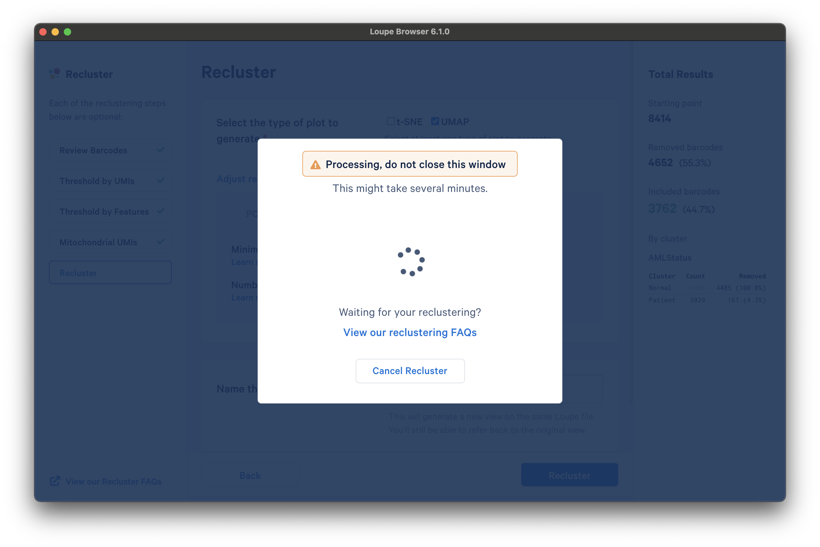
Run time will depend on your local machine speed, but is most dependent on the number of barcodes going into the reclustering, and whether you are running a t-SNE projection, a UMAP projection, or both. If only generating a single projection, expect most datasets under 10,000 cells to reprocess in less than two minutes. Larger datasets above 30,000 cells may take over 10 minutes, and there is a hard cap at 100,000 cells. Datasets near that 100,000-cell limit may take nearly an hour to process. Generating both a t-SNE and a UMAP projection will double the processing time. To reduce run time, consider only generating a UMAP projection, which will complete in roughly half the time compared to a t-SNE projection for datasets of 20,000 cells and above.
Once the reclustering is complete, you should see the following:
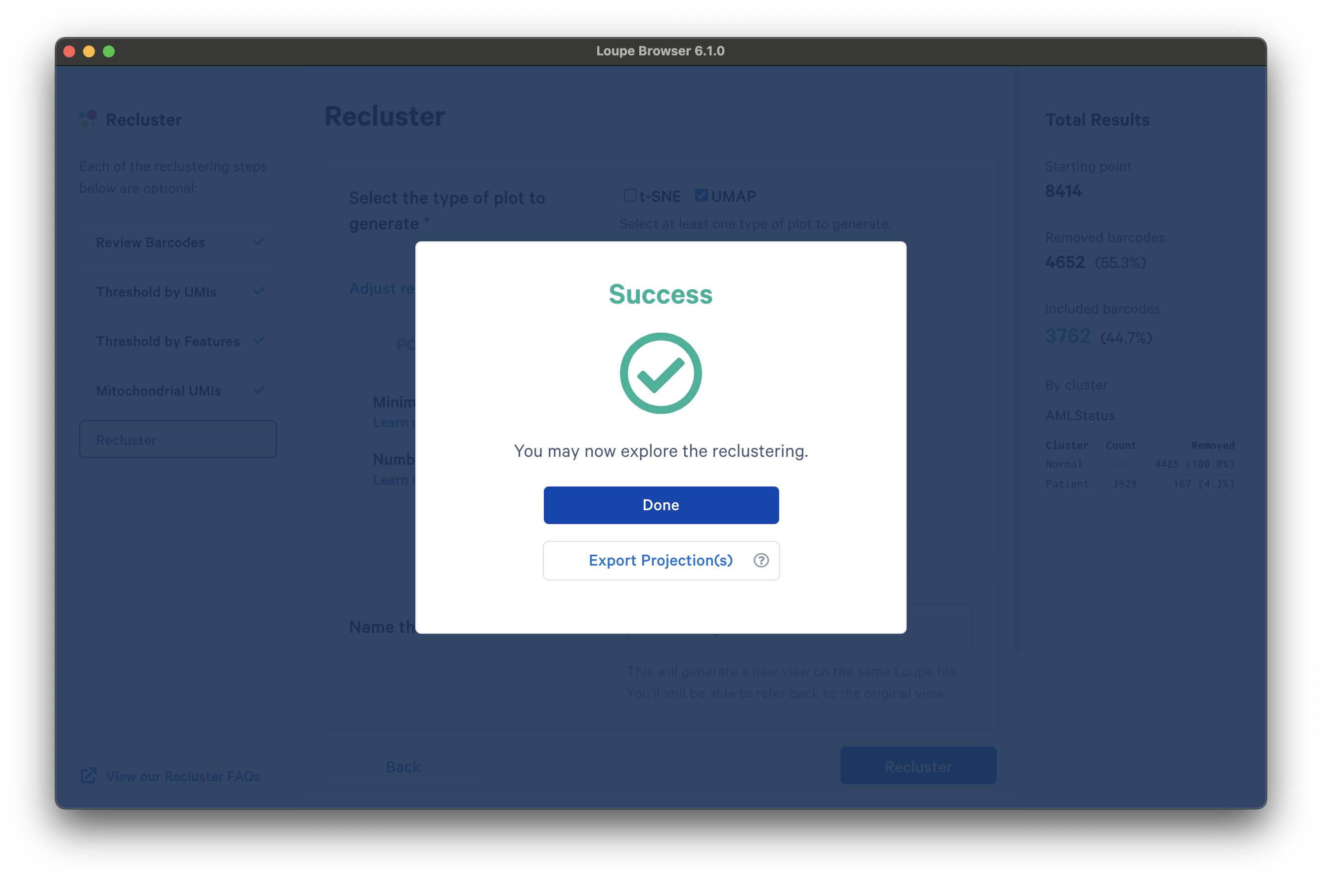
At this stage, in Loupe Browser 6.0 and later, you can export a CSV file with the projection coordinates for the t-SNE and/or UMAP projection(s) that were generated from this window by clicking Export Projection(s).
When reclustering completes, click on the Done button, which will close the workflow window, and bring up the new projection and category in the main window. You can now find it under a separate Analysis category in the View Selector menu. You can also export the projection CSV file by clicking the three vertical dots on the View Selector for each plot type. The AML Tutorial PatientOnly dataset is shown below:
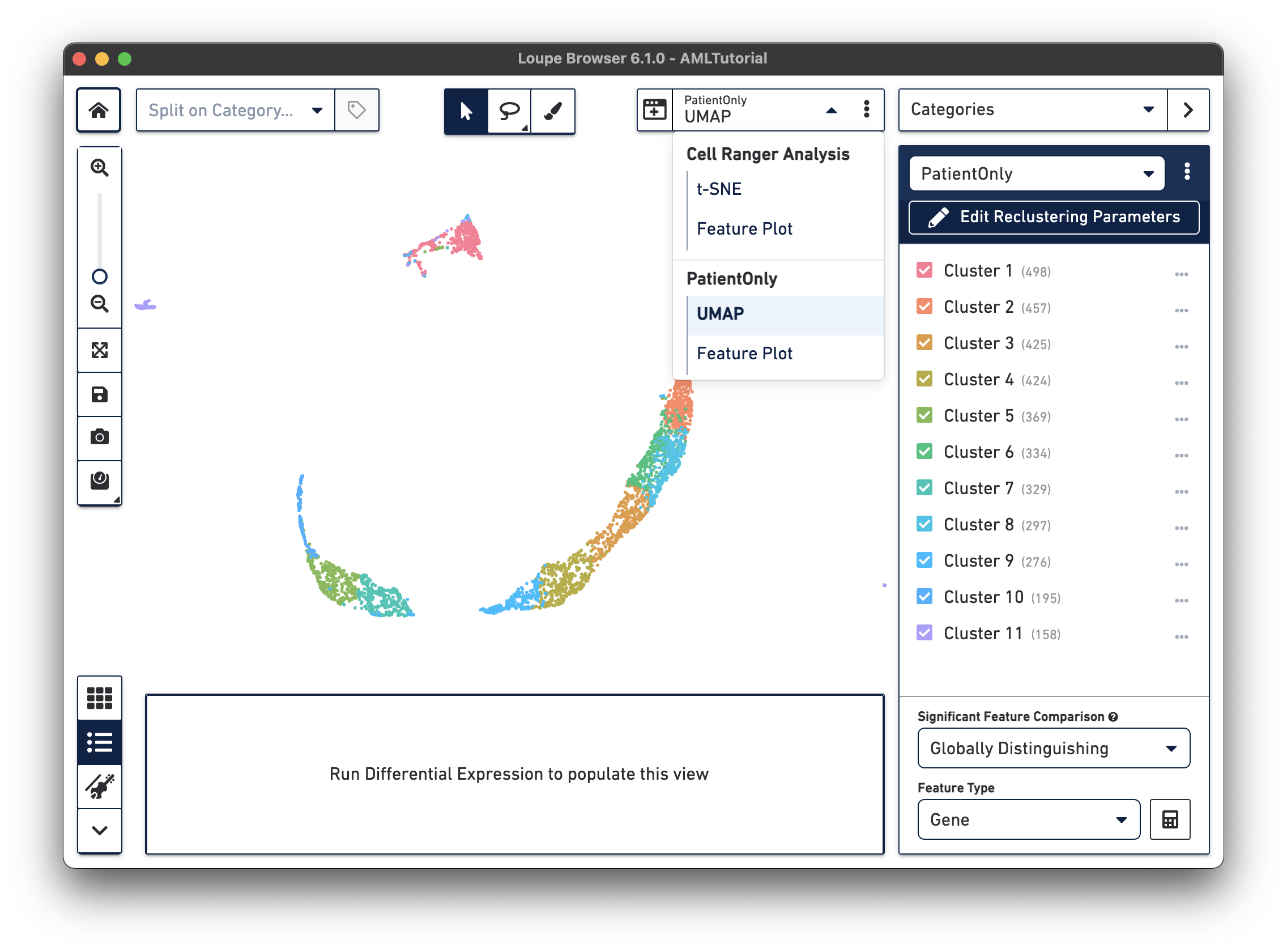
All operations in Loupe done while the reclustering-derived projection is visible will be limited to the barcodes in that projection. It is possible to look up significant genes limited to the reclustered barcodes, see gene expression projections with that cell subset, as well as see clonotype lists limited to the active barcode set. In addition, selecting a category derived from a reclustering will automatically load the projection associated with that reclustering. However, it is still possible to change projections while a reclustering-derived category is active, to see how the recomputed clusters map onto the larger data.
Saving the .cloupe at this time will save the reclustered projections and categories
only (though not any computed differential expression data). Finally, it is possible
to either tweak the reclustering or recall its parameters by clicking on the
Edit Reclustering Parameters button, located below any reclustered category.
Which 10x Genomics products can I filter and recluster?
How many cells can I recluster? Are there any limits?
Does reclustering recompute the PCA?
What type of projection does reclustering generate (e.g. t-SNE, UMAP)?
Why is reclustering taking so long?
How do I specify mitochondrial genes for the Mitochondrial UMI filter step?
How can I provide feedback or feature requests related to reclustering?