Cell Ranger7.1, printed on 03/03/2025
The computational pipeline cellranger count or multi for 3' Single Cell Gene Expression involves the following analysis steps:

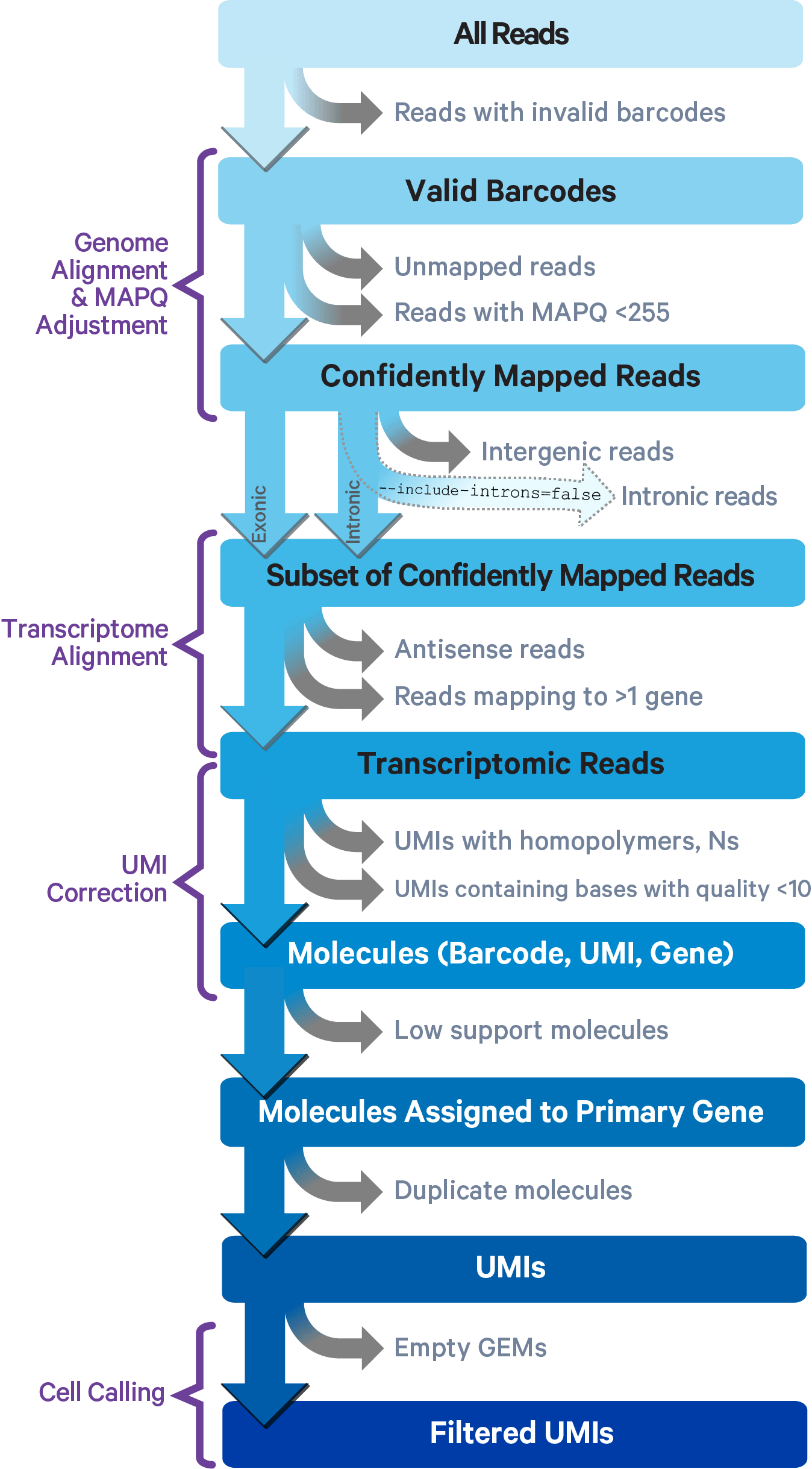
The key read processing steps are outlined in this figure and described in the text below:
This section on read trimming applies to 3' gene expression assays.
A full length cDNA construct is flanked by the 30 bp template switch oligo (TSO) sequence, AAGCAGTGGTATCAACGCAGAGTACATGGG, on the 5' end and poly-A on the 3' end. Some fraction of sequencing reads are expected to contain either or both of these sequences, depending on the fragment size distribution of the sequencing library. Reads derived from short RNA molecules are more likely to contain either or both TSO and poly-A sequence than longer RNA molecules.
Since the presence of non-template sequence in the form of either TSO or poly-A, low-complexity ends confound read mapping, TSO sequence is trimmed from the 5' end of read 2 and poly-A is trimmed from the 3' end prior to alignment. Trimming improves the sensitivity of the assay as well as the computational efficiency of the software pipeline.
Tags ts:i and pa:i in the output BAM files indicate the number of TSO nucleotides trimmed from the 5' end of read 2 and the number of poly-A nucleotides trimmed from the 3' end. The trimmed bases are present in the sequence of the BAM record, and the CIGAR string shows the position of these soft-clipped sequences.
Cell Ranger uses an aligner called STAR, which performs splicing-aware alignment of reads to the genome. Cell Ranger then uses the transcript annotation GTF to bucket the reads into exonic, intronic, and intergenic, and by whether the reads align (confidently) to the genome. A read is exonic if at least 50% of it intersects an exon, intronic if it is non-exonic and intersects an intron, and intergenic otherwise.
For reads that align to a single exonic locus but also align to 1 or more non-exonic loci, the exonic locus is prioritized and the read is considered to be confidently mapped to the exonic locus with MAPQ 255.
Cell Ranger further aligns confidently mapped exonic and intronic reads to annotated transcripts by examining their compatibility with the transcriptome. As shown below, reads are classified based on whether they are exonic (light blue) or intronic (red) and whether they are sense or antisense (purple).
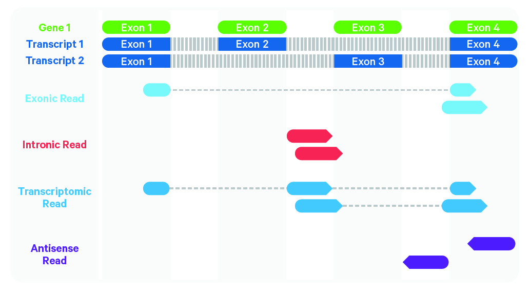
Starting in Cell Ranger 7.0, by default, the cellranger count and cellranger multi pipelines will include intronic reads for whole transcriptome gene expression analysis. Any reads that map in the sense orientation to a single gene - the reads labeled transcriptomic (blue) in the diagram above - are carried forward to UMI counting. Cell Ranger ignores antisense reads (purple). As shown above, antisense reads are defined as any read with alignments to an entire gene on the opposite strand and no sense alignments. Consequently, the web summary metrics "Reads Mapped Confidently to Transcriptome" and "Reads Mapped Antisense to Gene" will reflect reads mapped confidently to exonic regions, as well as intronic regions. The default setting that includes intronic reads is recommended to maximize sensitivity, for example in cases where the input to the assay consists of nuclei, as there may be high levels of intronic reads generated by unspliced transcripts.
To exclude intronic reads, include-introns must be set to false. In this case, Cell Ranger still uses transcriptomic (blue) reads with sense alignments (and ignores antisense alignments) for UMI counting, however a read is now classified as antisense if it has any alignments to a transcript exon on the opposite strand and no sense alignments.
| The include-introns option eliminates the need for a custom "pre-mRNA" reference that defines the entire gene body to be an exon. |
Furthermore, a read is considered uniquely mapping if it is compatible with only a single gene. Only uniquely mapping reads are carried forward to UMI counting (see this page for methods to check for multi-mapped reads).
| Note, in the Web Summary HTML, the set of reads carried forward to UMI counting is referred to as "Reads mapped confidently to transcriptome". |
To determine whether barcode sequence is correct, Cell Ranger compares 10x Barcodes to the known barcodes for a given assay chemistry, which are stored in a barcode whitelist file. For example, there are roughly 737,000 barcodes in the whitelist for the Single Cell 3' v2 and V(D)J assays, and ~3 million barcodes for the Single Cell 3' v3 and v3.1 chemistries.
Cell Ranger uses the following algorithm to correct putative barcode sequences against the whitelist:
The corrected barcodes are used for all downstream analysis and output files. In the output BAM file, the original uncorrected barcode is encoded in the CR tag, and the corrected barcode sequence is encoded in the CB tag. Reads that cannot be assigned a corrected barcode will not have a CB tag.
Before counting UMIs, Cell Ranger attempts to correct for sequencing errors in the UMI sequences. Reads that were confidently mapped to the transcriptome are placed into groups that share the same barcode, UMI, and gene annotation. If two groups of reads have the same barcode and gene, but their UMIs differ by a single base (i.e., are one Hamming distance apart), then one of the UMIs was likely introduced by a substitution error in sequencing. In this case, the UMI of the less-supported read group is corrected to the UMI with higher support.
Cell Ranger again groups the reads by barcode, UMI (possibly corrected), and gene annotation. If two or more groups of reads have the same barcode and UMI, but different gene annotations, the gene annotation with the most supporting reads is kept for UMI counting, and the other read groups are discarded. In case of a tie for maximal read support, all read groups are discarded, as the gene cannot be confidently assigned.
After these two filtering steps, each observed barcode, UMI, gene combination is recorded as a UMI count in the unfiltered feature-barcode matrix. The number of reads supporting each counted UMI is also recorded in the molecule info file.
Cell Ranger v3.0 and later have an improved cell-calling algorithm that is better able to identify populations of low RNA content cells, especially when low RNA content cells are mixed into a population of high RNA content cells. For example, tumor samples often contain large tumor cells mixed with smaller tumor infiltrating lymphocytes (TIL) and researchers may be particularly interested in the TIL population. The new algorithm is based on the EmptyDrops method (Lun et al., 2019).
The algorithm has two key steps:
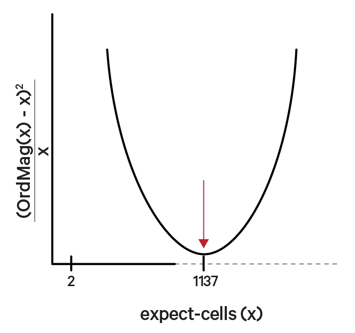
In the first step, the original Cell Ranger cell calling algorithm is used to identify the primary mode of high RNA content cells, using a cutoff based on the total UMI count for each barcode. Cell Ranger may take as input an expected number of recovered cells (e.g., see --expect-cells for count), N, or as of Cell Ranger 7.0, estimate this number.
The order of magnitude algorithm (OrdMag) estimates the initial number of recovered cells such that barcodes are called cells if total UMI counts exceed m/10, where m is the 99th percentile of top N barcodes based on total UMI counts. The estimation of expect-cells then finds a value x that approximates OrdMag(x) by minimizing a loss function where expect-cells = minx(OrdMag(x) - x)2 / x. Cell Ranger's grid-search goes from 2 to ~45k cells. In the example below, the optimized value for expect-cells is 1,137:
In the second step, a set of barcodes with low UMI counts that likely represent "empty" GEM partitions is selected. A model of the RNA profile of selected barcodes is created. This model, called the background model, is a multinomial distribution over genes. It uses Simple Good-Turing smoothing to provide a non-zero model estimate for genes that were not observed in the representative empty GEM set. Finally, the RNA profile of each barcode not called as a cell in the first step is compared to the background model. Barcodes whose RNA profile strongly disagrees with the background model are added to the set of positive cell calls. This second step identifies cells that are clearly distinguishable from the profile of empty GEMs, even though they may have much lower RNA content than the largest cells in the experiment.
Below is an example of a challenging cell calling scenario where 300 high RNA content 293T cells are mixed with 2,000 low RNA content PBMC cells. On the left is the cell calling result with the cell calling algorithm prior to Cell Ranger 3.0 and on the right is the Cell Ranger 3.0 result. You can see that low RNA content cells are successfully identified by the new algorithm.
 |
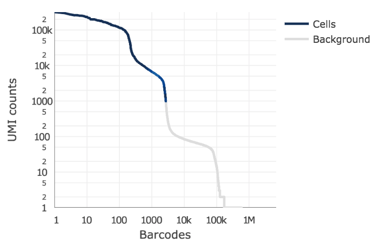 |
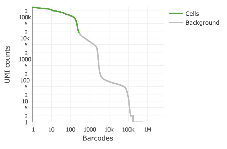
The plot shows the count of filtered UMIs mapped to each barcode. Barcodes can be determined to be cell-associated based on their UMI count or by their RNA profiles. Therefore some regions of the graph can contain both cell-associated and background-associated barcodes. The color of the graph represents the local density of barcodes that are cell-associated.
In some cases the set of barcodes called as cells may not match the desired set of barcodes based on visual inspection. This can be remedied by either re-running count or reanalyze with the --force-cells option, or by selecting the desired barcodes from the raw feature-barcode matrix in downstream analysis. Custom barcode selection can also be done by specifying --barcodes to reanalyze.
| Starting with Cell Ranger 6.1, the dynamic range of possible cell loads on the Chromium X Series, including LT and HT kits, is 100 - 60,000 cells. Occasionally, the previous default value of --expect-cells (3,000) may not have been adequate for optimal cell calling because --expect-cells was based on detecting barcodes within an order of magnitude of an anchor barcode. Starting from Cell Ranger 7.0, --expect-cells can either be auto-estimated or provided with a reasonable estimate of recovered cells. |
Cell Ranger 4.0 includes a new dedicated cell calling algorithm that is applied specifically to identify cells from Targeted Gene Expression datasets. The Targeted Gene Expression cell calling method relies on identification of a transition point based on the shape of the barcode rank plot to separate cell-associated barcodes from background partitions, and is designed to successfully classify cells for a wide variety of potential target gene panels.
Note: This method is distinct from the cell calling algorithm used for non-targeted Whole Transcriptome Analysis (WTA) {{platform.name}} single cell datasets, and it does not employ the EmptyDrops approach (Lun et al., 2019) due to the distinct features of Targeted Gene Expression datasets.
When using Cell Ranger in Feature Barcode Only Analysis mode, only step 1 of the cell calling algorithm is used. The cells called by this step of the algorithm are returned directly.
When multiple genomes are present in the reference (for example, Human and Mouse, or any other pair), Cell Ranger runs a special multi-genome analysis to detect barcodes associated with partitions where cells from two different genomes were present. Among all barcodes called as cell-associated (See Calling cell barcodes), they are initially classified as Human or Mouse by which genome has more total UMI counts for that barcode. Barcodes with total UMI counts that exceed the 10th percentile of the distributions for both Human and Mouse are called as observed multiplets. Because Cell Ranger can only observe the (Human, Mouse) multiplets, it computes an inferred multiplet rate by estimating the total number of multiplets (including (Human, Human) and (Mouse, Mouse)). This is done by estimating via maximum likelihood the total number of multiplet GEMs from the observed multiplets and the inferred ratio of Human to Mouse cells. If this ratio is 1:1, the inferred multiplet rate is approximately twice the observed (Human, Mouse) multiplets.
In order to reduce the gene expression matrix to its most important features, Cell Ranger uses Principal Components Analysis (PCA) to change the dimensionality of the dataset from (cells x genes) to (cells x M) where M is a user-selectable number of principal components (via num_principal_comps). The pipeline uses a python implementation of IRLBA algorithm, (Baglama & Reichel, 2005), which we modified to reduce memory consumption. The reanalyze pipeline allows the user to further reduce the data by randomly subsampling the cells and/or selecting genes by their dispersion across the dataset. Note that if the data contains Feature Barcode data, only the gene expression data will be used for PCA and subsequent analysis.
For visualizing data in 2-d space, Cell Ranger passes the PCA-reduced data into t-SNE (t-Stochastic Neighbor Embedding), a nonlinear dimensionality reduction method (Van der Maaten, 2014). The C++ reference implementation by Van der Maaten (2014) was modified to take a PRNG seed for determinism and to expose various parameters which can be changed in reanalyze. We also decreased its runtime by fixing the number of output dimensions at compile time to 2 or 3.
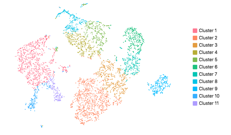
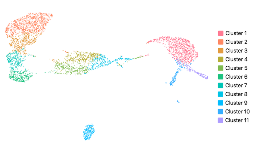
Cell Ranger also supports visualization with UMAP (Uniform Manifold Approximation and Projection), which estimates a topology of the high dimensional data and uses this information to estimate a low dimensional embedding that preserves relationships present in the data (McInnes et al, 2018). The pipeline uses the python implementation of this algorithm by McInnes et al (2018). The reanalyze pipeline allows the user to customize the parameters for the UMAP, including n_neighbors, min_dist and metric etc. Below shows the t-SNE (left) and UMAP (right) visualizations of our public dataset 5k PBMCs.
 |
 |
Cell Ranger uses two different methods for clustering cells by expression similarity, both of which operate in the PCA space.
The graph-based clustering algorithm consists of building a sparse nearest-neighbor graph (where cells are linked if they among the k nearest Euclidean neighbors of one another), followed by Louvain Modularity Optimization (LMO; Blondel, Guillaume, Lambiotte, & Lefebvre, 2008), an algorithm which seeks to find highly-connected "modules" in the graph. The value of k, the number of nearest neighbors, is set to scale logarithmically with the number of cells. An additional cluster-merging step is done to perform hierarchical clustering on the cluster-medoids in PCA space and merge pairs of sibling clusters if there are no genes differentially expressed between them (with B-H adjusted p-value below 0.05). The hierarchical clustering and merging is repeated until there are no more cluster-pairs to merge.
The use of LMO to cluster cells was inspired by a similar method in the R package Seurat.
Cell Ranger also performs traditional K-means clustering across a range of K values, where K is the preset number of clusters. In the web summary prior to 1.3.0, the default selected value of K is that which yields the best Davies-Bouldin Index, a rough measure of clustering quality.
In order to identify genes whose expression is specific to each cluster, Cell Ranger tests, for each gene and each cluster i, whether the mean expression in cluster i differs from the mean expression across all other cells.
For cluster i, the mean expression of a feature is calculated as the total number of UMIs from that feature in cluster i divided by the sum of the size factors for cells in cluster i. The size factor for each cell is the total UMI count in that cell divided by the median UMI count per cell (across all cells). The mean expression outside of cluster i is calculated in the same way. The log2 fold-change of expression in cluster i relative to other clusters is the log2 ratio of mean expression within cluster i and outside of cluster i. When computing the log2 fold-change, a pseudocount of 1 is added to both the numerator and denominator of the mean expression.
To test for differences in mean expression between groups of cells, Cell Ranger uses the exact negative binomial test proposed by the authors of the sSeq method (Yu, Huber, & Vitek, 2013). When the counts become large, Cell Ranger switches to the fast asymptotic negative binomial test used in edgeR (Robinson & Smyth, 2007).
Note that Cell Ranger's implementation differs slightly from the sSeq paper: the size factors are calculated using total UMI count instead of using DESeq's geometric mean-based definition of library size. As with sSeq, normalization is implicit in that the per-cell size factor parameter is incorporated as a factor in the exact and asymptotic probability calculations.
To correct the batch effects between chemistries, Cell Ranger uses an algorithm based on mutual nearest neighbors (MNN; Haghverdi et al, 2018) to identify similar cell subpopulations between batches. The mutual nearest neighbor is defined as a pair of cells from two different batches that is contained in each other’s set of nearest neighbors. The MNNs are detected for every pair of user-defined batches to balance among batches, as proposed in (Polanski et al, 2020).
The cell subpopulation matches between batches will then be used to merge multiple batches together (Hie et al, 2019). The difference in expression values between cells in a MNN pair provides an estimate of the batch effect. A correction vector for each cell is obtained as a weighted average of the estimated batch effects, where a Gaussian kernel function up-weights matching vectors belonging to nearby points (Haghverdi et al, 2018).
The batch effect score is defined to quantitatively measure the batch effect before and after correction. For every cell, we calculate how many of its k nearest neighbors belong to the same batch, where k is the square root of the number of cells, and normalize it by the expected number of same batch cells when there is no batch effect. If there is no batch effect, we would expect that the nearest neighbors of each cell are evenly shared across all batches and the batch effect score is close to one. There is a batch effect if the batch effect score is greater than one. The batch effect score value is not comparable across experiments with different numbers and/or batch sizes.
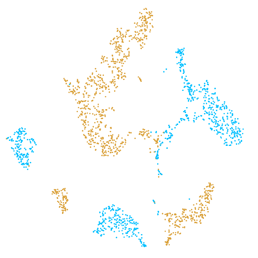
In the example below, the PBMC mixture was profiled separately by Single Cell 3' v2 (brown) and Single Cell 3' v3 (blue). On the left is the t-SNE plot after aggregating two libraries without the batch correction, and on the right is the t-SNE plot with the batch correction. The batch effect score decreased from 1.81 to 1.31 with the chemistry batch correction.
 |
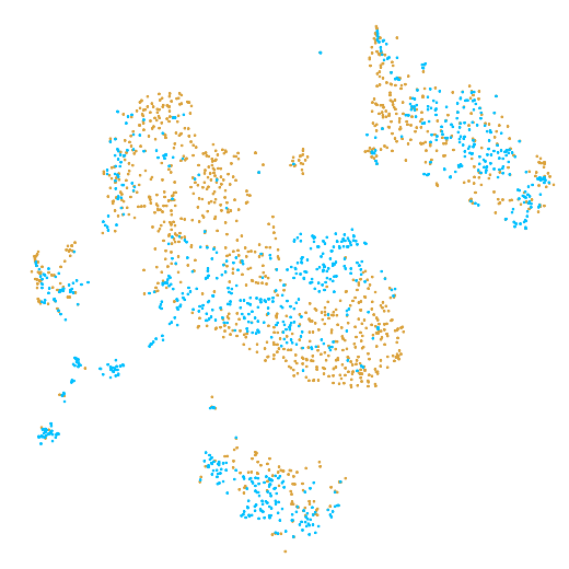 |
| Note that the feature-barcode matrix is not adjusted by Chemistry Batch Correction. |
Baglama J and Reichel L. Augmented implicitly restarted Lanczos bidiagonalization methods. SIAM Journal on Scientific Computing 27: 19–42, 2005.
Blondel V, et al. Fast unfolding of communities in large networks. Journal of Statistical Mechanics: Theory and Experiment, 2008.
Haghverdi L, et al. Batch effects in single-cell RNA-sequencing data are corrected by matching mutual nearest neighbors. Nature Biotechnology 36, 2018.
Hie B, Bryson B, and Berger B. Efficient integration of heterogeneous single-cell transcriptomes using Scanorama. Nature Biotechnology 37: 685-691, 2019.
Lun A, et al. Distinguishing cells from empty droplets in droplet-based single-cell RNA sequencing data. Genome Biology 20, 2019.
McInnes L, Healy J, and Melville J. UMAP: Uniform Manifold Approximation and Projection for dimension reduction. arXiv, 2018.
Polanski K, et al. BBKNN: fast batch alignment of single cell transcriptomes. Bioinformatics 36: 964-965, 2020.
Robinson M and Smyth G. Small-sample estimation of negative binomial dispersion, with applications to SAGE data. Biostatistics 9: 321–332, 2007. Link to edgeR source.
Van der Maaten, LJP. Accelerating t-SNE using tree-based algorithms. Journal of Machine Learning Research 15: 3221-3245, 2014.
Yu D, Huber W, and Vitek O. Shrinkage estimation of dispersion in Negative Binomial models for RNA-seq experiments with small sample size. Bioinformatics 29: 1275–1282, 2013.